Running a simulation#

A simulation combines a medium or waveguide, a temporal grid, an input pulse, nonlinear responses and numerical settings. Choose these from the physical question, then save enough information to check the result. The introductory RDW and soliton lessons take this sequence from parameters through plots and interpretation.

This chapter explains the entry points and how to configure a simulation before running it. Continue to accessing and continuing a run for output, progress and logging for diagnostics, and execution resources for memory and threads.

There are three ways in, and they are the same machinery underneath:

the keyword interfaces prop_gnlse() (a solid-core fibre described by its dispersion and nonlinear coefficient), prop_capillary() (a gas-filled hollow capillary described by its radius, gas and pressure) and prop_waveguide() (a supplied set of gas-filled modes, or a guide that solves its own), which take the numbers a fibre is usually quoted with;
their constructors, from_gnlse(), from_capillary() and from_waveguide(), which build the same simulation without running it;
the object Simulation itself, which takes the physics objects directly.

Free-space and planar propagation have entry points of their own, prop_radial(), prop_free() and prop_planar(), described on the free-space chapter. They use the same output, continuation, progress and resource controls linked above.

The numerical settings control the error of the chosen discrete problem. They do not certify the physical model or the spatial and temporal resolution. Plan convergence checks around the observables you intend to report.

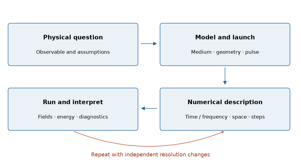
A workflow from physical question to model, grid and launch, propagation, and analysis, with a return arrow for independent convergence checks. — Setting up a simulation and assessing its result. A converged stepper answers the discrete problem you gave it; change the grid and spatial description separately to check whether that problem resolves the physics.#

One call#

from solprop.driver import prop_gnlse

output = prop_gnlse(
    0.11,                                   # gamma, 1/(W m)
    1.33,                                   # fibre length, m
    [0.0, 0.0, -11.83e-27],                 # beta_0, beta_1, beta_2 about wavelength
    wavelength=835e-9,
    wavelength_limits=(500e-9, 2e-6),
    trange=4e-12,
    width=100e-15,                          # the natural width of a sech**2
    peak_power=96.8,
    shape="sech",
    rtol=1e-9,
    n_save=201,
)

That builds an envelope grid, maps gamma onto a third-order susceptibility, wraps the Taylor coefficients in a dispersion-specified mode (SpecifiedMode), builds the input pulse, selects the backend, propagates the pulse and stores 201 planes. It returns the Output it wrote — here a MemoryOutput, because no output was given.

Units are SI throughout (conventions.md §1), with one exception at the interface: loss_db_per_m is in decibels per metre, as a data sheet quotes it, and is converted by attenuation_from_db(). (Pressures, on the gas-filled routes below, are in bar.)

The step control is reached through rtol, atol, dz_init and dz_max on every entry point. Unless told otherwise, prop_gnlse steps with RungeKutta() at rtol=1e-7 and atol=1e-14 (in √W), prop_capillary with Multistep() at 1e-6 and 1e-10, and prop_waveguide with RungeKutta() at 1e-5 and 1e-10. Each interface takes the integrator SEP 37 measured fastest at matched accuracy on its benchmark cases, except the capillary, which keeps the Adams method by the maintainer’s decision, and the loosest tolerance that passed SEP 37’s convergence test with it (the defaults). The first trial step is length * 1e-4 and the longest allowed is half the fibre unless dz_init and dz_max say otherwise. These are starting points: the error a local tolerance buys at the output depends on the problem, so calibrate it (the solver). A schedule= replaces the adaptive stepping by a fixed schedule (fixed schedules).

The GNLSE is not a separate solver path. It is the mode-averaged envelope problem with a mode whose beta(omega) is given rather than derived, density = 1, prefactor_index = 1, and the shock term supplied by the omega dependence of the normalisation prefactor (the GNLSE page).

Three keywords change what is modelled rather than how it is stepped. shock=False freezes that omega dependence, which is what makes the equation the plain nonlinear Schrödinger equation whose N-soliton solutions are exact. raman=True gives raman_fraction (by default optmat’s silica bundle’s, 0.2188) of the nonlinear coefficient to a fused-silica Raman response and leaves the rest with the Kerr term, which is what produces the soliton self-frequency shift. It is off by default in prop_gnlse, and with it off the whole of gamma acts as Kerr unless raman_fraction is given, which is held back either way (the GNLSE page). polarisation_taper=True tapers the nonlinear polarisation inside the spectral collar (the band just outside the active band where the field is absorbed, see boundaries); it is off by default because the rate absorber already acts on the field there, and the taper costs a systematic error of the size of the field’s content in the collar.

pulses=[...] launches several pulses together in place of the single-pulse keywords, for two-colour and multi-colour inputs, on every keyword entry point of this page (several pulses at once).

A table or mode as the GNLSE fibre#

Give exactly one of betas, beta and fibre, and one of gamma and n2. The first positional argument is still required, so pass None for it: prop_gnlse(None, length, fibre=table, n2=..., ...), or the equivalent Simulation.from_gnlse call. n2 requires a fibre with an effective area; a table’s area is evaluated at wavelength. With gamma, a table without an area uses 1 m². The mapping is gamma = n2 omega0 / (c A_eff) and chi3 = (4/3) (1 - f_R) n2 eps0 c, with unit prefactor index, the usual shock term and the requested silica Raman fraction \(f_R\); the GNLSE page derives the mapping under “The coefficient mapping”, including why raman=False omits the factor unless a fraction is given.

A supplied mode contributes dispersion, loss and mode.aeff() – or, for a general modal guide’s provider channel, its area solved again at wavelength (the GNLSE page). It is wrapped in SpecifiedMode.from_mode, whose frozen callables keep the original mode for reproducible records. Its fill is ignored as a nonlinear material: gamma or n2 supplies that physics, and the run’s configuration records the fibre as a GNLSE mode. Use the capillary route when a mode’s fill should drive the nonlinear responses.

A mode whose geometry moves – a tapered bore, a pressure gradient – is carried too, and both of its paths come with it: the frozen callables forward the position, so the dispersion and the loss are evaluated where they are asked for, and the effective area is sampled from the same mode over the positions its own declared paths kink at. There is no separate keyword and no second entry point; the GNLSE page has the model under “A varying dispersion, declared with the area”.

The fibre carries its loss, so any explicit loss_db_per_m beside it, including zero, is refused. Scale or replace loss on the supplied mode. Tables must cover every active-band frequency, including collars, and any derivative probes; extrapolation is refused. The tabulated-mode guide explains the area, loss interpolant and measured limits, and the gallery executes a synthetic solid-core GNLSE example.

A capillary, end to end#

prop_capillary() is the same shape as prop_gnlse and a different physics. It builds everything a gas-filled hollow fibre needs from the numbers such a fibre is quoted with:

from solprop.driver import prop_capillary

output = prop_capillary(
    125e-6,                                 # core radius, m
    1.5,                                    # length, m
    "He",
    (0.8, 0.0),                             # bar, entrance to exit: a gradient to vacuum
    wavelength=800e-9,
    wavelength_limits=(90e-9, 4e-6),
    trange=400e-15,
    fwhm=7.5e-15,
    energy=275e-6,
    modes=4,
)

That is resonant-dispersive-wave emission in a helium-filled capillary: a 7.5 fs, 275 µJ pulse at 800 nm self-compresses along a pressure gradient to vacuum and sheds a dispersive wave in the vacuum ultraviolet, and the first four HE₁ₘ modes carry it. This page calls it the RDW case below. The gallery runs a reduced version of it. Where the defaults of this interface differ from Luna.jl’s, the differences are listed in Noteworthy differences from Luna.

Gas mixtures. Pass a Mixture in the gas position and omit pressure, or pass a mapping such as {"N2": 0.8, "O2": 0.2} with a total pressure. The same ordered densities feed every mode and response. plasma={"N2": True, "O2": True} selects separate ionisation channels; preionisation={"O2": 0.01} sets only that component’s initial fraction, and a ZProfile in place of the number makes it a path along the fibre (nonlinear.md). By default the Raman response is on for every component with a validated optmat response, nitrogen and oxygen both; raman=("N2",) selects nitrogen alone, and an explicit selection of a component without data raises by name. Mixture.air(...) gives the explicitly normalised N₂/O₂/Ar composition, argon included; gas="air" with a total pressure is the two-component convenience, nitrogen and oxygen renormalised to each other with argon folded away (Mixture.air(..., argon=False)). See mixtures for independent profiles, total-loss controls, species statistics and saved-field analysis.

To change the fill of an existing simulation without rebuilding it, use with_mixture(): it takes a mixture with the same ordered labels and species and new paths or populations, and keeps the geometry, grid, input, noise and settings. The translated result shares the ionisation rate tables and the unchanged Raman kernels with the original and rebuilds only what depends on the new densities; what it reused is logged. This is the cheap way to scan pressure (scans). The spatial routes accept a mixture as SpatialMedium(material=mixture); on a Cartesian grid its density profiles must be constant.

Several things differ from prop_gnlse, and each is a modelling choice the keywords reach.

Field or envelope. The default is FieldGrid, which propagates the real electric field, with third-harmonic generation on. envelope=True selects the envelope grid and keeps both thg and plasma off by default. Explicit plasma=True or an instantaneous rate object on an envelope grid selects cycle-averaged envelope plasma, which cannot be combined with thg=True. It runs on numpy_ref and the native backend; a backend that cannot run a problem refuses it by name rather than falling back (the backend notes give the qualification of each).

A set of modes on one transverse quadrature. modes=4 is the first four HE₁ₘ modes of the capillary (he1m()); a sequence of modes is adopted as given and checked for orthonormality, since one synthesis matrix and its dual represent an orthonormal basis and nothing else. The transverse integral of the nonlinear polarisation is a fixed rule, never an adaptive one: the fixed Gauss or Gauss–Kronrod rule integrates Kerr and Raman overlaps accurately when its order resolves the mode profiles, converges spectrally for a smooth ionisation rate, and costs the same on every step, where an adaptive cubature’s cost depends on the field and its error estimate can be far too optimistic with a kinked rate. Its radial order n_r defaults to default_radial_order() of the mode count – 32 up to four modes, eight nodes per mode above that. radial_rule="gauss_kronrod", the default, makes the rule the Kronrod extension of the half-order Gauss rule, whose embedded Gauss subset costs nothing and gives the run an error estimate (the quadrature alarm, below). n_theta is refused for a set of HE₁ₘ modes: |J₀(u r/a)| does not depend on the angle, so every azimuthal node would be a copy of the same integrand.

A supplied mode set is the run’s geometry: the positional radius must agree with its modes’ core radius along the run, and a model, loss or cladding declared away from its default must be theirs, or the call is refused by name. It may contain TabulatedHollowMode (an evacuated table plus the declared gas) or TabulatedMode (one filled table’s whole index); the driver keeps their type and table while binding the declared mixture. Hollow tables support pressure gradients; filled tables require constant material paths matching the fill used to obtain their data. Both keep Marcatili transverse fields. With a table area, choose reference_wavelength explicitly; this fixes the area used in propagation.

A tube lattice. Pass lattice=TubeLattice(wall_thickness=180e-9, tube_radius=9e-6, n_tubes=6) beside an integer modes= to select the Vincetti model of an antiresonant fibre. The radius argument remains the core radius, while cladding is the tube material. lattice is refused with supplied modes or model="reduced". A supplied sequence of VincettiMode objects keeps its class and tube geometry when rebound to the declared gas mixture.

A run with no nonlinearity is refused for every mode set, tube lattice or capillary; a linear check builds a Simulation with an empty response sequence.

A coherent wall. By default each HE₁ₘ channel loses power through the capillary wall at its own Marcatili rate, independently of the others. wall=CoherentWall() replaces those independent losses by the condensed Robin boundary block: the outgoing boundary condition at the wall, condensed onto the retained modes, which couples every \(\mathrm{HE}_{1m}\) channel to every other with a definite phase and so converts a launch between them. On a taper or a pressure gradient it also carries the connection the moving basis costs. CoherentWall(impedance="te_tm") condenses the wall’s two impedances instead of their average, coupling the two radial families of one azimuthal order, on a straight bore or a taper alike. The block is the run’s loss model, so loss= must stay True; it needs the contiguous set modes=N builds (or one azimuthal order, for the te_tm block) and a scalar state, and it is refused beside lattice= and model="reduced", each by name. It carries the default input noise; the modified noise model is refused beside it. It runs on numpy_ref and the native backend, CPU and GPU builds alike, with the default integration method; CoherentWall(method="cf4"), which integrates each section by commutator-free exponentials of its whole generator, runs on numpy_ref alone. See the coherent wall, the capillary guide and the gallery examples they link.

The taper coupling. A multimode capillary whose radius varies along z carries the taper coupling by default, with or without a wall and lossless or not: the connection \(\langle\psi_m|\partial_z\psi_n\rangle\) that moves power between the HE₁ₘ channels as the bore changes. taper_coupling=False is the explicit opt-out to the adiabatic route, on which each channel follows its local mode and exchanges no power; it is refused beside a wall, which always carries the connection, and has no effect on one channel or a constant bore (the taper coupling without a wall). Like the wall, the coupling is a coupled flow on a field grid with one field component, and it refuses an envelope grid and the modified noise model by name; taper_coupling=False is the route for either. The input noise model is admitted: its draw is part of the launch, which the coupling propagates like any field.

A density that varies along the fibre. pressure is a number, a pair (p_in, p_out) for the steady-flow gradient p(z) = √(p₀² + z/L (p₁² − p₀²)), or a pair (z, p) of a staged fill, all in bar. On a taper the steady flow follows the bore (p² linear in ∫ a⁻⁴ dz), and an end pumped to vacuum is choked at the pressure where the laminar throughput equals the sonic one (vacuum_end="choked", the default); the fill warns if the flow is not laminar or not a continuum (profiles, solprop.gasflow). The same path drives both the modes’ core index and the responses’ density, so a gradient disperses and broadens consistently, and the density, the pressure and the core radius are recorded at every saved plane. With vacuum_end="floor" a fill keeps its declared ends (on a taper it still follows the bore); one that reaches a true vacuum then has dp/dz diverging at its end, so solprop floors it at 10⁻⁴ of the highest stage pressure unless pressure_floor says otherwise, and says so in the log. temperature (293.15 K by default, or a path along z) sets the density the pressure maps to.

Walk-off, warned about before the run. A mode set is written in one co-moving frame, the first mode’s (the linear operator), so the group delay between its modes is real: the fourth HE₁ₘ mode of the example above drifts 346 fs against the fundamental over its 1.5 m, whatever the fill. from_capillary integrates that spread along the fibre at the reference frequency and asks warn_walkoff() whether the temporal collar can absorb a packet crossing it that slowly. The 400 fs window above can; a 100 fs one cannot, and the warning then names the wider window or the stronger absorber that would.

Plasma. plasma=True, the default on a field grid, tabulates an ionisation rate over the fields the run will reach: optmat’s recommended rate model of each species at the carrier; the ionisation manual describes the models and their limits. An explicit rate object overrides selection, for example plasma=OptmatRate("H2", 800e-9, model="moadk_zhao_2010") after importing OptmatRate from solprop.nonlinear.optmat_rates. plasma=False disables it, and envelope runs default to no plasma. The span of the table comes from the input’s own peak field, over the axis and the run’s transverse nodes (the axis for an HE_1m launch, the nodes for a TE_0m or TM_0m one, whose field vanishes on the axis), unless ionisation_field_range gives one – default_field_range() explains the two factors. Above the upper limit the table holds its last value, so one set too low is a silent clip of the rate exactly where ionisation matters; below the lower one the rate is zero, which is where every rate in this package already is.

Raman, for a molecular fill. By default (raman=None) a molecular fill with a validated optmat response – N₂, O₂, H₂, D₂, CH₄ and SF₆, and air through its nitrogen and oxygen – carries optmat’s rotational and vibrational response of the gas (Raman responses from optmat), which is absolute: there is no raman_fraction here, as there is for the normalised fibre model of prop_gnlse, whose own default is raman=False. An atom carries no Raman response and says nothing; a molecule whose response is provisional (N₂O) warns and goes without, unless MaterialSelection(raman="provisional") admits it; raman=False switches it off, and so does kerr=False, a deliberately reduced model. raman=True on a noble gas is refused by name, and raman=True without kerr=True is refused too: a medium with a Raman response has an electronic one as well, and on a field grid the drive form reaches the kernel through the Kerr term (raman). The run’s temperature sets the rotational populations, the same number the density path and the mode set are built at. The same default holds for prop_waveguide().

Four statistics only a backend can compute. Beside the multimode defaults and the z-profiles, a capillary run records the electron density, the peak ionisation rate, the peak on-axis intensity and the quadrature error – the difference between the fixed rule’s projection and its embedded coarse one. That last is an alarm, never a controller input: above QUADRATURE_ALARM (\(10^{-6}\)) the backend logs once per plane and the run continues, because a rule that cannot resolve the integrand is not something a smaller step can fix; raise n_r instead. On four HE₁ₘ modes at the default order its largest value in the RDW case is 1.0×10⁻⁶. See statistics.

The introductory RDW lesson reports its current parameters, runtime and quadrature diagnostic. The RDW convergence study uses the singular true-vacuum endpoint, so its convergence rates do not describe the default choked fill or establish convergence of a different simulation. A true-vacuum end (vacuum_end="floor" with pressure_floor=0.0) makes dp/dz diverge: it is the one place the step controller cannot meet its tolerance, and the observed convergence order falls to about one. Prefer the default choked end (vacuum_end="choked"), which stops the fill at a finite pressure. Always vary step tolerance, temporal sampling and spatial resolution separately.

Configure before running#

Simulation is what prop_gnlse builds. Use it directly when the physics is not a GNLSE fibre, or when one configuration is to be run more than once:

from solprop.driver import Simulation, SimulationSettings
from solprop.stepper import PIController

simulation = Simulation(
    grid,
    mode,
    [kerr],
    pulse,
    settings=SimulationSettings(
        controller=PIController(rtol=1e-9, atol=1e-18),
        save_planes=[0.25, 0.5, 0.75, 1.0],
        dz_max=0.1,
        dz_init=1e-4,
    ),
    noise=realisation,
    profiles={"density": path},
)

problem = simulation.translate()      # the kernel problem, built once and cached
memory = simulation.run()             # into memory
simulation.run("run.h5")              # and again, into a file, without translating twice

SimulationSettings holds everything numerical: the controller and its tolerances, the save planes, the step limits, a fixed schedule, the tableau, the absorber and how it is applied, the transverse quadrature, the statistics and the backend. translate() does everything expensive that does not depend on the state — the cumulative linear operator, the masks, the modal transform, the compiled responses — and caches it, so a second run of the same simulation reuses it. metadata() builds the record that says what produced a file, and caches it for the same reason: two runs of one simulation are the same run and must digest alike. with_input() and with_mixture() derive a new simulation with another input pulse or another fill while sharing what translation built (scans).

SimulationSettings.fields and field_planes choose which saved planes keep their field — every one by default, the named ones, or none for a run wanted as statistics alone (output). They are execution settings, outside the configuration hash, and may change after translation.

What a run will cost#

simulation.estimate() answers before a run: the state’s shape, the persistent memory its constructed backend holds, the output’s size for the planes and fields it keeps, the cost of one right-hand-side evaluation on its backend, timed after an untimed warm-up that takes the compilation and transform planning (reported as setup), and the integrator’s evaluations per step, with their total for a replayed schedule. It does not predict the number of adaptive steps, which the physics decides. It builds the backend, so a run that doesn’t fit in memory fails here as the run would.

Many inputs, one backend: the runner#

A large problem pays for its backend before it takes a step: about fifteen copies of the state are allocated and first touched, and the transforms are planned. A delay scan or a sweep of the input runs the same translated problem for hundreds of inputs, and need pay that once. runner() translates (or reuses the cached translation) and constructs one backend; each run() then loads one input into it and runs the save-plane loop (SEP 22 §5.2):

import dataclasses

simulation.settings = dataclasses.replace(simulation.settings, fields="none")
spectra = []
with simulation.runner() as runner:
    for delay in delays:
        output = runner.run(
            build_input(delay),                  # an array or a pulse, as with_input takes
            configuration={"delay": delay},      # recorded in this run's hash
            progress="none",
        )
        spectra.append(output["stats/on_axis_spectrum"])
# the backend is closed when the block ends; a closed runner refuses run()

Each run derives its input with with_input() and has its own record, configuration hash and handler: output= takes a handler or a path, and None gives a new MemoryOutput. Loading an input restores everything a march reads — the state, the controller, a dense observation’s look-ahead, the quadrature alarm, an Adams march’s history and call ledger (StepDriver.set_initial) — so a run on the reused backend repeats a fresh backend’s run, to the rounding that separates any two runs.

The runner checks that each input’s problem is the one its backend was built for, but for the input, and refuses by name:

a different launch position (initial_z): the save planes and the schedule’s cursor belong to the constructed problem;
a different noise model: the backend carries the one it was built with (noise="keep", the default, keeps the realisation; another realisation of the same model may be passed);
a run with a TDSE response, whose atomic binding has its own lifecycle;
a second run started while one is running: one backend steps one input at a time.

A run that raises leaves the runner open, since the next input resets everything; a backend that closed itself closes the runner.

The march holds no input. An array the record keeps by its digest (below) is read in place rather than copied, and the runner drops every reference to it, and to the launch a modal route converts it to, as soon as the backend has loaded it. So an input formed in the call, as above, is freed before the first step. Two arrays are kept all the same: a smaller array, which the record carries inline, is copied into it, and the simulation the runner was built from keeps its own input for as long as it lives. For a scan over large arrays, build that simulation from a broadcast, which holds one repeated block:

placeholder = np.broadcast_to(np.zeros((1, 1, 1), dtype=np.complex128), shape)
simulation = Simulation(grid, (), responses, placeholder, settings=settings, ...)

Spell the call’s keywords out too: when any argument is unpacked, Python keeps a call’s positional arguments for as long as the call runs, so runner.run(build_input(delay), **options) holds the input through the march, one volume.

with_input itself validates only what changed: the replaced input’s shape, dtype and one finiteness pass, and the replaced noise’s, with every other leaf of the translated problem shared rather than scanned again; a new initial_z keeps the stepper’s checks. Its configuration= merges caller keys into the derived run’s record (a key the run records itself is refused). An array input, here and in the constructor, is copied when the simulation is built, so changing it afterwards changes neither the run nor its record; an array input of more than 2²⁰ elements is recorded by the SHA-256 of its bytes rather than inline, so a gigabyte launch costs seconds of hashing per input rather than gigabytes of JSON.

A caller that already knows what its input is need not pay even that. Both with_input and SimulationRunner.run take input_identity=, a string the record then holds with the array’s dtype and shape (StatedInput) in place of the array’s own record, without reading its bytes, so the run’s hash follows the string:

output = runner.run(
    build_input(delay),
    input_identity=f"pump {pump_label}, delay {delay:.6e} s",
    progress="none",
)

Warning

An identity is taken on trust. Two different arrays stated alike have one configuration hash, so a wrong identity passes a resume and a scan’s cache: the resumed run or the cached point is then the wrong one, and nothing can tell. Say everything that makes the input what it is, and leave input_identity out unless the digest is a measured cost.

Only an array can be stated; a pulse is a small record of itself and is refused. A file written with a statement is continued only under the same statement, not by the same array without one, since the two records differ. The finiteness pass stays: it costs a few percent of a digest, about 0.6 s and 9 s for a 4 GiB input on a Xeon without SHA instructions, and it refuses a bad input before it is loaded.

The boundary check on a free-space scan. The default boundary_check reads a free-space run’s transverse edge on the host at the launch, at every plane and at every read: it copies the state across and transforms it out of place, even with fields="none". That is about 1.1 field volumes more at the peak, which neither memory_ledger nor the admission counts, and on native CPU at 256 × 256 × 96 with two planes it took a point from 0.96 to 2.1 volumes above the level before the input, and from 3.05 to 3.99 s. A scan whose window is already settled can pass boundary_check=None. That also turns off the check of the time window’s edges, since no setting keeps one without the other, so settle the window on one input with the check on first.