A radially symmetric beam under the Kerr effect#

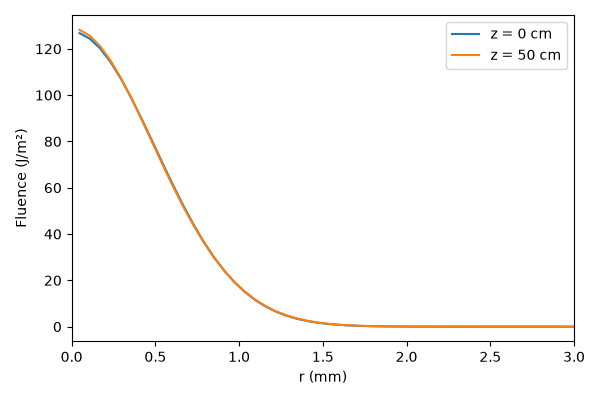
A collimated 800 nm, 30 fs beam of 1 mm waist and 0.2 mJ, in 1 bar of argon, on a radial (Hankel) grid, below the critical power for self-focusing. Over 50 cm the Kerr lens offsets about half of the beam’s diffraction: its second-moment radius grows by 0.45 %, where diffraction alone (a Rayleigh length of 3.9 m) gives 0.81 %. The run is a plain prop_radial(), every argument an object a recipe writes as a table, and it is the call the radial route’s example recipe mirrors (Recipe.example("radial_kerr")).

The chart is the fluence across the beam at the entrance and after 50 cm.

from time import perf_counter

import matplotlib.pyplot as plt
import numpy as np

from solprop.driver import SimulationSettings, prop_radial
from solprop.grid import EnvelopeGrid, RadialGrid
from solprop.nonlinear.responses import KerrResponse
from solprop.physdata import gamma3
from solprop.pulses import GaussianPulse, SpatialPulse
from solprop.spatial import SpatialFlux, SpatialMedium, spatial_fluence
from solprop.stats import StatsSpec
from solprop.stepper import PIController

started = perf_counter()

The run#

The aperture is four waists, 64 radial samples; the envelope grid leaves out the third harmonic. Five planes are saved along the 50 cm, the energy and the beam radius recorded at each.

length = 0.5
grid = EnvelopeGrid.from_limits(length, 800e-9, (600e-9, 1100e-9), 200e-15, thg=False)
space = RadialGrid(4e-3, 64)
argon = SpatialMedium("Ar", pressure=1.0)
settings = SimulationSettings(
    controller=PIController(rtol=1e-5, atol=1e-12),
    save_planes=[0.1, 0.2, 0.3, 0.4, 0.5],
    dz_init=0.01,
    dz_max=0.05,
    stats=StatsSpec(names=("energy", "beam_radius")),
)
result = prop_radial(
    grid,
    space,
    argon,
    [KerrResponse(gamma3("Ar", wavelength=800e-9), thg=False)],
    SpatialPulse(GaussianPulse(wavelength=800e-9, fwhm=30e-15, energy=2e-4), 1e-3),
    settings=settings,
    noise=None,
)

The fluence across the beam#

The fluence through each plane in the argon, against the radius.

figure, axis = plt.subplots(figsize=(6, 4))
for index, z in ((0, 0.0), (-1, length)):
    plane = SpatialFlux.resolve(grid, space, argon, z=z)
    fluence = spatial_fluence(result.fields("fft")[index], plane)
    axis.plot(space.r * 1e3, fluence, label=f"z = {z * 100:.0f} cm")
axis.set(xlabel="r (mm)", ylabel="Fluence (J/m²)", xlim=(0, 3))
axis.legend()
figure.tight_layout()
# The second-moment radius (the statistic's first column, the 1/e^2 radius the second).
radius = np.asarray(result["stats/beam_radius"])[:, 0] * 1e3
print(f"Second-moment radius: {radius[0]:.4f} mm -> {radius[-1]:.4f} mm")
print(f"Complete radial Kerr example: {perf_counter() - started:.3f} s")

Second-moment radius: 1.0000 mm -> 1.0045 mm
Complete radial Kerr example: 1.013 s

A radially symmetric beam under the Kerr effect#

The run#

The fluence across the beam#

Related reading#